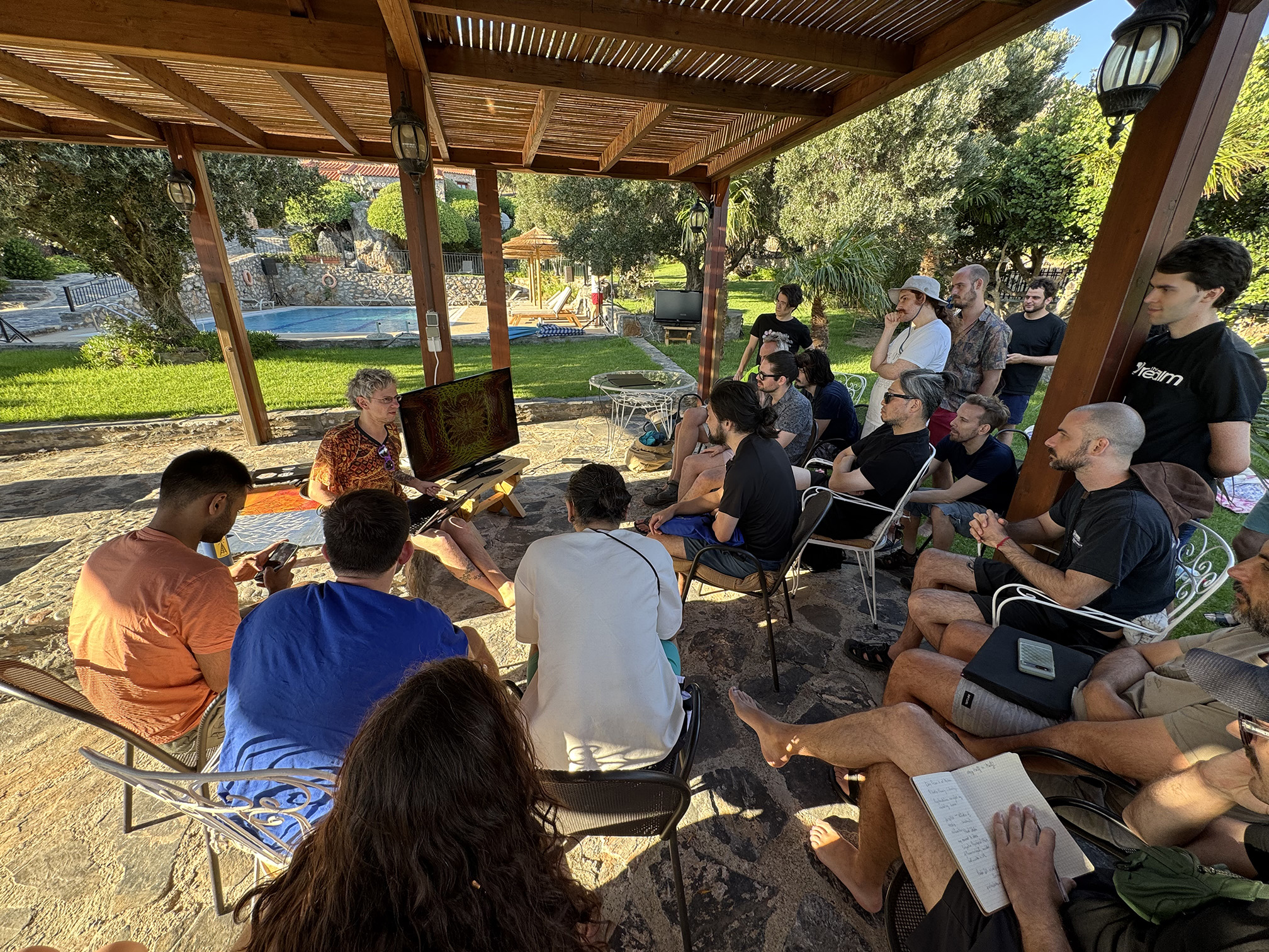
The visual artist Symmetric Vision giving a presentation on his psychedelic replication technique to a crowd of psychedelic and meditation researchers at the QUALIUS retreat.
The formless jhāna or arūpa jhāna are the final four out of the series of eight concentration states known as the jhāna. They are named as such for their lack of form, i.e. heterogeneous sensations such as a body map – whatever their structure may be, in order for it to be formless it must be homogeneous. As an experienced meditator progresses from J5 to J8, they generally report experiencing increasingly abstract states – until they achieve complete cessation of experience altogether.
Previously, at The Science of Consciousness Conference 2025, I met with Niffe Hermansson, who proposed that J8 corresponded to the instantiation of time – given that the sensation of time passing was the only thing which differentiated J8 from cessation. When I related this to Ethan, he expanded on this; in his eyes, J8 corresponded to the more mathematically fundamental notion of continuity – in the formal, epsilon-delta definition sense.
I myself am not an accomplished meditator and do not have any direct insight into what these states are like. Something which perplexed me was the problem of how someone might even analyse such states from the inside, given that metacognition itself is generally completely absent during such states of consciousness. Ethan claimed that in order to report on their internals, you have to set yourself up such that the structure of these interior states can be inferred from the outside by the changes imparted on subjective experience after the fact. Wystan was later able to clarify this for me – depending on the degree of absorption, one might have some amount of cognitive maneuverability, but in more highly absorbed states, one is restricted to observing the state via the memories that are accessible afterwards.
I felt more comfortable taking these reports at face value now that I understood the chain of causality which produced them. To this end, I found myself hauling Ethan through a laborious, from first principles infodump on these highly abstract states over the course of several hours. In order to describe the principles he believes each successive jhāna adds to experience, he used sufficiently general mathematical language that I could wrap my head around what he was saying. A brief sketch of the preliminary model he outlined during this conversation is as follows:
J8: Neither perception or non-perception
Continuity. Just continuity; continuity is the only thing that differentiates J8 from full cessation. Continuity implies open sets; points have neighbourhoods.
J7: Boundless nothingness
Accumulation and dissolution. Note that this is not the sense of accumulation or dissolution; you have the sense of continuity, but there are no absolute quantities, just first differentials. Not Turing complete.
J6: Boundless consciousness
Comparison and reflection. Objects reflect one another, they can be compared, but the relative time delays have not assembled themselves into a sense of space.
J5: Boundless space
Space. Reflections congeal into a sense of space. The construction of independence. You have the hologram for the first time; there’s just nothing in it.
Hang on, I said. Do you see it? My immediate impression was that these seemed an awful lot like an instruction set or at least a set of computational primitives employed by some kind of general purpose analog computer.
Typically the jhāna are described as a progression from waking consciousness all the way to cessation. However, if we start with cessation and work backwards through J8 to J1, under this model it seems more like we are progressively adding various computational properties to consciousness, until we arrive at something more like day-to-day experience. Now – what if we could also find a physical structure or process within the brain which accumulates equivalent computational properties as consciousness boots up from cessation – what would that tell us about consciousness?
So, what are we actually doing here? Resuming a top-down perspective, I still consider myself to be investigating how consciousness works. I see the translation problem, as specified by Mike Johnson, to be one of the key problems to which any theory of consciousness must propose a solution. As outlined in a previous post:
In Mike’s book, Principia Qualia, he attempts to decompose the problem of consciousness into a programme of subproblems, one of which he calls the translation problem. This asks, by which psychophysical laws do physical states map onto qualia states, and vice versa? This is closely related to David Chalmers’ combination problem:
The Translation Problem: given a mathematical object isomorphic to a system’s phenomenology, how do we populate a translation list between its mathematical properties and the part of phenomenology each property or pattern corresponds to?
Or more succinctly, how do we connect the quantitative with the qualitative?
Recently, I discussed this problem with the philosopher David Pearce. He also sees the translation problem as one of the key problems of consciousness, but, in his own words, without some kind of cosmic Rosetta Stone, our prospects remain hopeless:
The world is formally described, exhaustively, by the equations of mathematical physics. But the essence of the physical isn’t what materialist metaphysicians suppose.
Nevertheless, consciousness mystifies me. For science lacks a cosmic Rosetta Stone to let us “read off” the myriad interdependent textures (“what it feels like”) of experience from the diverse solutions to the equations of quantum field theory.
Could the jhāna provide such a Rosetta Stone for consciousness? For some time now, I’ve seen psychedelic drugs as a viable tool for investigating consciousness, but while they are very good at perturbing consciousness in a way that reveals its dynamics, I have somewhat given up hope that psychedelics can reliably lead to the kind of repeatable, convergent states which could bridge between phenomenological reports and neuroimaging studies. This said, it seems that the jhāna provide a set of consistent concentration states across a variety of contemplative traditions. Insofar as they might be natural attractor states within human nervous systems, perhaps the jhāna could provide such a psychophysical bridge?
Despite decades of progress in the neuroscience of consciousness, prevailing empirical paradigms remain largely anchored in the study of typical, content-rich states that are characterized by layered perceptual, cognitive, affective, and self-referential processes. Such complexity may obscure the neural mechanisms that give rise to conscious experience. Here, we propose that advanced meditation – referring to states and stages of practice that unfold progressively with increasing expertise – offers a powerful yet unexplored opportunity to isolate the core features of consciousness through a theory-driven neuroscience approach.
We focus on two classes of meditative phenomena: advanced concentrative absorption (related to what have been called jhāna), which involves the preservation of highly abstract forms of awareness alongside the attenuation of typical features of consciousness; and meditative endpoints – namely, cessation events (related to what have been called nirodha) – which involve the temporary suspension of consciousness altogether. These phenomena serve as precise, replicable, and experimentally tractable phenomenological anchors for a minimal model framework, a novel approach aimed at identifying and characterizing the simplest possible form of conscious experience as a principled starting point for a systematic science of consciousness. Within this framework, the integration of advanced meditation into experimental paradigms offers a promising path toward identifying the neural mechanisms that support consciousness in its most reduced and fundamental forms.
The Meditation Research Program has recently published the first case study of ultra–high-field fMRI of jhāna, with the first group-level study currently in preprint, plus two single-subject reanalyses of the case study dataset applying connectivity gradient and geometric eigenmode decompositions:
I find all this very inspiring. At our end, we don’t have the kind of resources they have at Harvard, but I took Ethan’s model to Andrés Gómez Emilsson at the Qualia Research Institute and suggested it was an excellent line into the translation problem. Several months later, here we are, fresh out of a jhāna retreat in Tepoztlán, México – and I have a small dataset of questionnaires and candid interviews with jhāna practitioners to work with. Abridged transcripts from those post-retreat interviews alongside additional commentary are available at:
The rest of this post will cover a review of the jhāna models which Ethan came up with during the retreat. We’re not settled on any one thing or another; to be perfectly clear, we’re proposing a set of complementary prototypes, which we can iterate on over time as we accumulate more reports and the state of neuroscience improves.
Typical late night scene in Tepoztlán: I was out of my depth and arranged for Ethan Kuntz to compare experiences with Wystan Bryant-Scott, after I interviewed Wystan earlier that same day.
Before we start, however, I’d like to review what we see as the primary challenges to this research:
Finding meditators who are literate in advanced mathematics
Priming issues from discussing models with meditators prior to experiences
Asking analog computers to report on their internal states when they are close to being shut down
First of all, it’s really hard to find people who can both jhāna and discuss abstract mathematical models of experience. Recently, I spoke with a well-known meditation teacher who ostensibly knew their mathematics – only to be met with confusion when I began speculating about the frequency domain properties of pīti and sukha. If you do think you could hold such a cross-domain conversation, we would be overjoyed if you got in touch.
Secondly, any contributor to this project will need to understand both mathematics and their own phenomenology well enough to be able to hold a model while not crushing their worldview into it. There exist academic interview standards – such as micro-phenomenology – which are designed to avoid asking leading questions of study participants. While I’m incredibly impressed with the quantity and quality of information such techniques can solicit, the models we are proposing are sufficiently specific that there’s really no way for them to pass through that kind of communication bottleneck. Contributors will need to be trusted to hold any models we invoke lightly enough to avoid both priming issues during experiences and post-hoc confabulation. We also need to be able to trust contributors to tell us if our models don’t square with your experience – until we’re confident enough in a given model that we know exactly what kind of psychophysics tests should verify what we propose. As Ethan suggested:
If we’re correct, this should be extremely demonstrable. If there’s really something here, it’s crisp – and if we’re right about this there will be ways to demonstrate this very strongly which pretty much obviate priming worries.
Thirdly, we’re asking people to report on remarkably subtle and easily overlooked aspects of experience. Like I mentioned earlier, there’s not a lot of metacognition to work with – as absorption deepens, self-reflection is progressively attenuated. I get the impression that it’s a little like trying to report accurately from inside an illucid daydream – as mentioned earlier, you only have the memories to work with from immediately after the state collapses. It’s almost like we are asking an analog operating system to log its own state while it shuts down as many of its processes as it can.
Though we began the retreat with a focus on anthropic analog computing, there was a large variety of other models that myself and Ethan played around with during our time in Tepoztlán. In this section, I shall run through four models of the form jhāna that we discussed. Perhaps the reader will find some of these lenses more relatable than others. In my research, I like to employ an attitude of many models, loosely held, and we’re very much applying this mindset here. Additionally, as Ethan said – we are optimistic that these may be all one model with many faces.
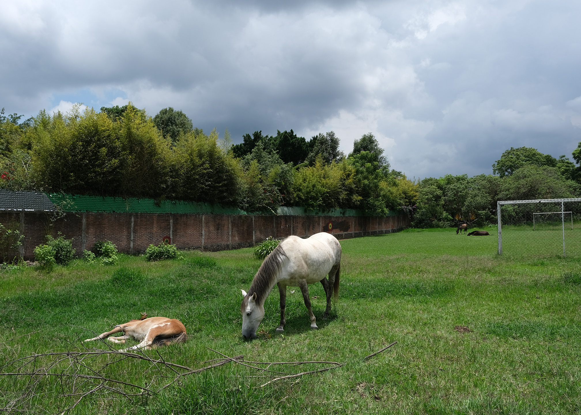
Typical daytime scene in Tepoztlán: Ethan and myself spent many long hours pacing the length of a nearby football field, discussing various models of the jhāna. Sometimes, there were horses.
Only four participants were able to access all four form jhāna, so be aware that our sample size is fairly small. This said, our participants’ reports were robust, and we felt confident in the trends we did observe. As I wrote, in The third QRI psychophysics retreat, part I: The form jhāna:
We observed two macroscale phenomenological trends across the form jhāna:
The pīti-sukha trend, in which different form jhāna are reported to have consistent relative proportions of pīti and sukha.
The head, heart, gut, everywhere trend, in which different form jhāna are reported to be accessible by concentrating attention in specific locations in the body.
As I understand, these pretty much square with what’s documented in the literature.
I’ll review these two trends, along with two additional models that Ethan proposed, in the following sections. First of all, let’s put these four models side by side to see if any patterns leap out:
There was a clear trend across the form jhāna which related to the relative proportions of the jhānic factors of pīti and sukha. I described these briefly here:
Of these jhāna factors, I find pīti and sukha to be of specific interest, as they describe two families of somatic textures which can arise within the body map either during meditation or in waking life. They can be quite pleasurable, and are also useful for identification of specific form jhāna states. I’ll save the speculation for a later post, but my general understanding is that pīti has heterogeneous microstructure described as noisy and powdery, whereas sukha has homogeneous microstructure described as smooth and creamy.
At one point, I thought to ask Wystan if he considered that the different jhāna could be characterised exclusively in terms of pīti and sukha:
Cube Flipper: Are the qualitative changes between J1 and J2 primarily characterised by the changes to pīti and sukha and their distributions in the body? Is there anything else you think characterised it?
Wystan: Not really.
Cube Flipper: Is it the same for the next one? And all the way through the form realms?
Wystan: Yes – it’s really just changes in the dynamics of pīti and sukha.
Participants generally reported the presence of pīti and sukha in the following relative proportions:
Ethan was happy to corroborate this on the record:
Cube Flipper: Can you explain what you think the trends are with regards to pīti and sukha?
Ethan: If I was to describe how I think other people will describe it and how this will fit into typical models: J1, basically all pīti. J2, nearly all sukha. J3, actually pure sukha. J4, neither.
We are not entirely sure why these factors present in the following proportions, but that’s what people consistently report. There’s an obvious parallel with the tetralemma model, which is quite curious. Before we go much deeper, perhaps we need to figure out what pīti and sukha actually are, first. Throughout the form jhāna post, we discussed the following models:
Pīti and sukha as fields of oscillations with phase-uncorrelated and phase-correlated phase, respectively – the order parameter from statistical mechanics is the quantity that tells these apart.
Pīti and sukha as signals with high spatiotemporal certainty and high spectral certainty, respectively – or rather, signals whose spread is smeared in the spectral domain and spatiotemporal domain, respectively.
Pīti and sukha as the building blocks of the somatic field, with pīti like a Gaussian or even Gabor splat and sukha like Grossbergian filling-in – or in less technical terms, point particles and smooth surfaces.
Pīti as noisy oscillations and sukha as the marginal background structure left over after those oscillations are dissolved – the motivating pleasant state used as an evolutionary reward mechanism.
Pīti and sukha as comparable to the effects of nitrous and codeine, respectively.
Pīti and sukha as mechanical and heat energy, respectively.
Pīti and sukha as difference and similarity, respectively.
The other trend which our participants reported semi-consistently is what we came to call the head, heart, gut, everywhere trend, in which pīti and sukha either initially present themselves in a specific bodily location – or are actively triggered when attention is placed on a specific bodily location:
J4: Absence of pīti and sukha everywhere; sometimes triggered by moving attention down the body and out through the floor
Alternatively – as Wystan often reported – if pīti and sukha did not localise to these specific locations, then generally they would pervade the bodymind uniformly instead.
I’ll confess that I don’t really think of the jhāna as something belonging to contemplative practices. Rather, if you think of nervous systems as resonant systems, I think that a good working hypothesis is to model the jhāna as outlier, low-entropy resonant modes which nervous systems can navigate into and inhabit by accident. Leigh Brasington reports in Right Concentration that about 10% of his students, upon encountering descriptions of the jhāna, recognise them as something they discovered how to do as children. Unless there’s something special about human nervous systems, I’d be surprised if other vertebrates and perhaps other animals in general did not also inhabit equivalent attractor states.
Evolution must surely be strongly incentivised to prevent organisms from accidentally getting sucked into trance states at inopportune moments, but it also suggests to me that there must be something special about the jhāna given that evolutionary incentives have not completely blocked their access. I suspect that modifying a nervous system in this way would sacrifice some other desirable qualities it possesses.
Returning to the head, heart, gut, everywhere pattern – I have to wonder if an animal with a drastically different body map would experience a different set of jhāna, or if these attractor states are more universal than that? What kind of jhāna might a fish or a centipede be able to access? As Wystan reports, in deeper absorption states, the jhāna can be experienced independent of the presence of a body map, with pīti-sukha flooding the entirety of subjective space. Does this suggest that indeed the form jhāna are natural kinds?
Ethan proposed that we could use some well-known field equations to describe the changes which the different jhāna make to the texture of experience. Imagine applying these to the phenomenal fields, where u is the intensity of the field at each point in spacetime:
We are effectively asking the reader to imagine how it would feel if they were to apply these field equations to their somatic field. What phenomenal textures might arise? This might be difficult to visualise, so we made a couple of renderings to illustrate the dynamics:
Field equations one to four applied to the same input field. J1 rings, J2 blurs fine detail first, J3 settles to a constant curvature equilibrium, and J4 dissolves large scale structure first, leaving fine detail. Please note that J3 and J4 crossfade from their initial conditions over the first second to avoid a jarring discontinuity.
Perhaps if you have first hand experience of the form jhāna this will be impressionistically relatable – or maybe it won’t. Ethan explained his model to me during our post-retreat interview:
Ethan: I have a sequence of extremely generic things that I think the brain uses a lot. We’ve got the wave equation, the heat equation, Poisson’s equation, and one quirky thing.
Cube Flipper: All right, okay.
Ethan: I would say that J1 is very wave equation, and J2 is very heat equation. One important thing is that the heat equation is the first derivative of intensity with respect to time – which is equal to the Laplacian of your intensity. Then the wave equation is just the second derivative which is equal to that – you just integrate one time. Stuff like this is one of the reasons I think that the jhāna are probably really genuinely crisp things.
Cube Flipper: Okay.
Ethan: One of the things about the heat equation – you get smoothing. You get diffusion. Very cool. The heat equation is the diffusion equation is mean curvature flow – the thing that J2 is doing is just minimizing curvature, locally and everywhere. These are all the same thing! This is really important.
Cube Flipper: Wystan describes smoothing his body map out using sukha. That’s the mean curvature flow thing?
Ethan: Yes.
Cube Flipper: Oh, interesting.
Ethan:J3. You know how we go from J1 to J2 by taking off a temporal derivative on intensity? We just do that again! The equation now – constant equals Laplacian. Mean curvature is constant everywhere. You know what that is? A constant mean curvature surface – like a soap bubble. You know what else this is? This is the steady state of some function whose Laplacian gives you your charge distribution. This is the steady state of an electric field.
Cube Flipper: Does J4 fit into this model?
Ethan:J4 is wacky. J4 is weird. When we’re in J3, we have fixed boundary conditions, upon which the mean curvature can’t actually be zero. In J4, we say, no. The boundary conditions can shift – everything can change, and change relative to everything else. There’s a progressive and deepening relaxation of the boundary conditions such that we’re actually going for zero.
Cube Flipper: Okay. That actually makes sense to me.
Ethan: There’s a repeated integration over the whole system such that we have to satisfy some constant curvature, and then the whole experience factors this out, and then we’re back to zero… or some distribution of charge or whatever. And then, rinse and repeat – you’ll asymptote to zero form. Then at some point, you get tired of this process, and you’re like, this is never going to end if I don’t just give up form entirely. So then you’re like, fuck form. I’m on to formless. It’s formless time. Then you’re on to the formless jhāna.
I believe that Ethan is working on a full writeup of this theory, so stay tuned. Personally, I’ll admit to finding this description pretty abstract, and light on phenomenological justification.
What we can do is try to compare this model to the descriptions which the other participants provided during their own post-retreat interviews. Those can be read in full in my retreat report – but I can also highlight some of the ways people tended to describe the form jhāna. I’ll let you decide if you think these relate to the field equations as shown:
The same four field equation applied to a standing wave rather than travelling wave pattern. Here, J1 oscillates in place rather than radiating outwards. This may be a better match for the phenomenology of pīti, which is more commonly described as noisy or buzzing.
We reviewed this relationship, considering whether there might also be something analogous in the formless jhāna:
Cube Flipper: Walking through the wave equation, heat equation, Poisson’s – you’re removing various features of that differential equation – it reminds me of removing computational operations in the case of the formless jhāna.
Ethan: Yeah, when you move up, you’re integrating in time.
Cube Flipper: How so? Can you explain that?
Ethan: For the wave equation, you have got the second temporal derivative equal to the spatial Laplacian. Heat equation, you’ve got the first temporal derivative equal to the spatial Laplacian. With J3, you have something static, where it’s just equal to this temporal thing. With J4, I suspect that you have an integral equal to this instead.
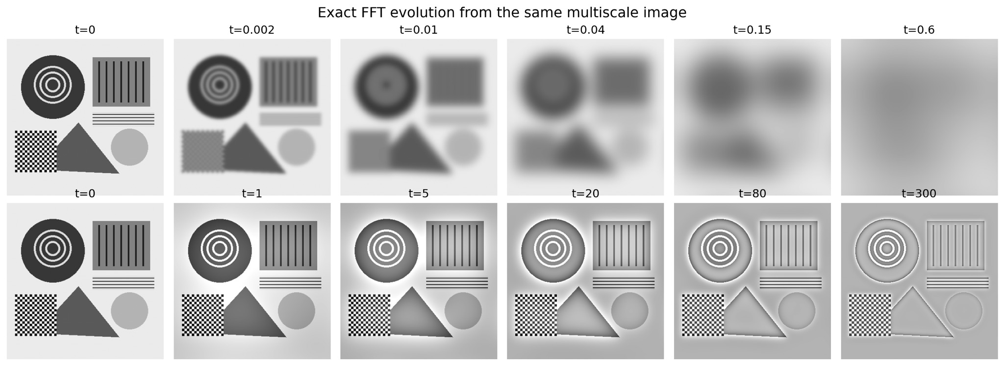
So, J1, J2, and J3 follow the pattern ∂nu/∂tn = ∇2u for n = 2, 1, 0 – and then J4 is the odd one out. Something worth noting in the case of J4 is how ∫ u dτ = ∇2u differentiates to ∂u/∂t = ∇−2u, the inverse Laplacian, which effectively runs the heat equation’s smoothing in reverse order. Where J2 smooths out fine structure and leaves coarse structure standing, J4 erases coarse structure and leaves fine structure standing. In this sense, J2 and J4 behave like a spatial low-pass filter and high-pass filter, respectively.
These images demonstrate repeated application of the proposed field equations for J2 and J4 to an example field. Note how J4 can behave like an edge detector. I wonder where I’ve seen that before. Images by Ethan Kuntz.
I was curious why this sequence terminates where it does. Why no 3rd derivative? I chatted to my OpenClaw agent Nix (Fable 5.1), who suggested that the answer would become apparent if we looked at what each field equation does to the field’s modes:
All four field equations share the same spatial eigenfunctions – the modes of the Laplacian, ∇2φ = −k2φ, where k is the wavenumber of the mode (small k for large-scale structure, large k for fine detail). Any field u is built as a sum of these modes, each with its own amplitude a(t). The four equations differ only in what time does to those amplitudes:
J1 modes ring: a ∝ e±ikt
J2 modes smooth: a ∝ e−k2t, so fine detail decays first and large-scale structure last
J3 modes hold: a is constant
J4 modes dissolve: a ∝ e−t/k2, so large-scale structure decays first and fine detail last
J2 and J4 are mirror images across J3 – one eats the top of the spectrum, the other the bottom – with J3 as the fixed point in between. That is what relaxing the boundary conditions looks like mode by mode, since the boundary is the largest-scale structure there is.
Why no third derivative? Per mode, the ladder reads ∂na/∂tn = −k2a. For n = 2 the characteristic roots are ±ik, pure oscillation. For n = 1 the root is −k2, pure decay. For n ≥ 3, the roots of rn = −k2 always include one with positive real part, so every mode has an exponentially growing solution. Orders one and two are the only ones where every mode stays bounded. This is the general fact behind the Ostrogradsky instability, and the Abraham–Lorentz self-force is its famous casualty – the top of the ladder is capped for the same reason Newtonian mechanics stops at acceleration.
I found this a fairly reasonable answer. It also helped me understand a modification to one of my models which Ethan had proposed – given that pīti and sukha together look like a Gabor wavelet:
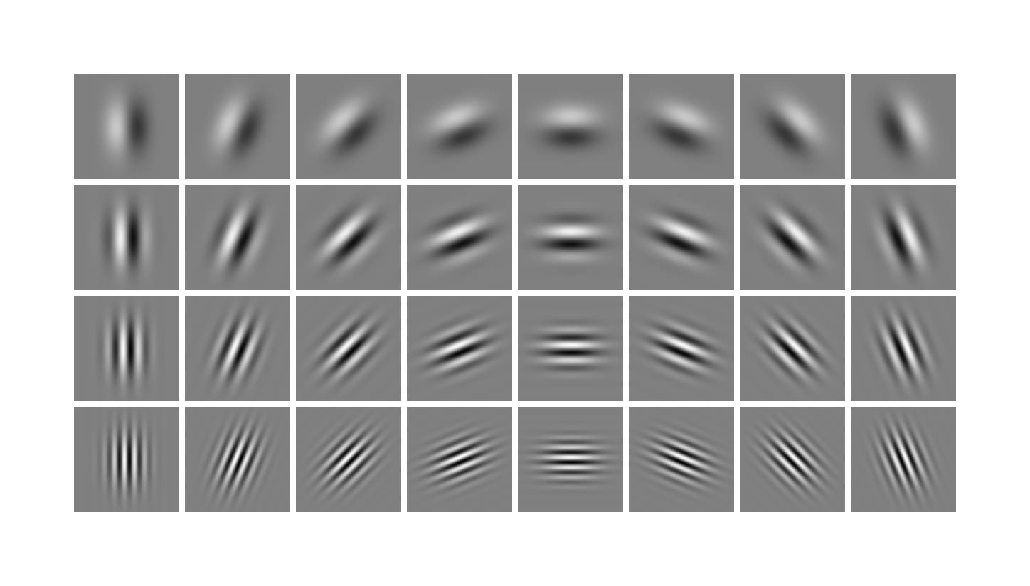
Ethan: One of the reasons I like the wave and heat distinction between pīti and sukha is because it also matches the Gabor wavelet quite nicely. The spatial eigenfunctions of the wave equation are sinusoids – very cool – and the spatial eigenfunctions of the heat equation are also just sinusoids. It’s the heat kernel that’s a Gaussian. Then the product of a sinusoid and a Gaussian is our Gabor patch.
Perhaps this is what the aforementionedbuilding blocks of experience look like – an oscillating J1 mode, masked by the Gaussian envelope from an impulse of J2.
A family of Gabor functions – sinusoids masked by Gaussians. Spatial frequency increases from top to bottom; orientation starts at 0° on the left and increases by 22.5° per column.
In contrast with the form jhāna, the formless jhāna are characterised by their lack of – well – form, which we take to mean anything which can be said to have a definite, formed shape within experience, be it visual, auditory, or somatic. In most situations we are talking about the presence of the body map, though this might also include incredibly subtle aspects of experience – for instance, someone might not notice that they are still rendering the sense of the walls in the room in which they are meditating. Wystan tells me that for J5, that has to go.
For this reason, the formless jhāna have significantly simpler structure than the form jhāna, and this is why we see them as much more viable Rosetta Stone candidates, and so we spent proportionally more time thinking about them. However, only three of our participants could access the formless jhāna, so, again, be aware that the set of reports which informs our models is fairly small.
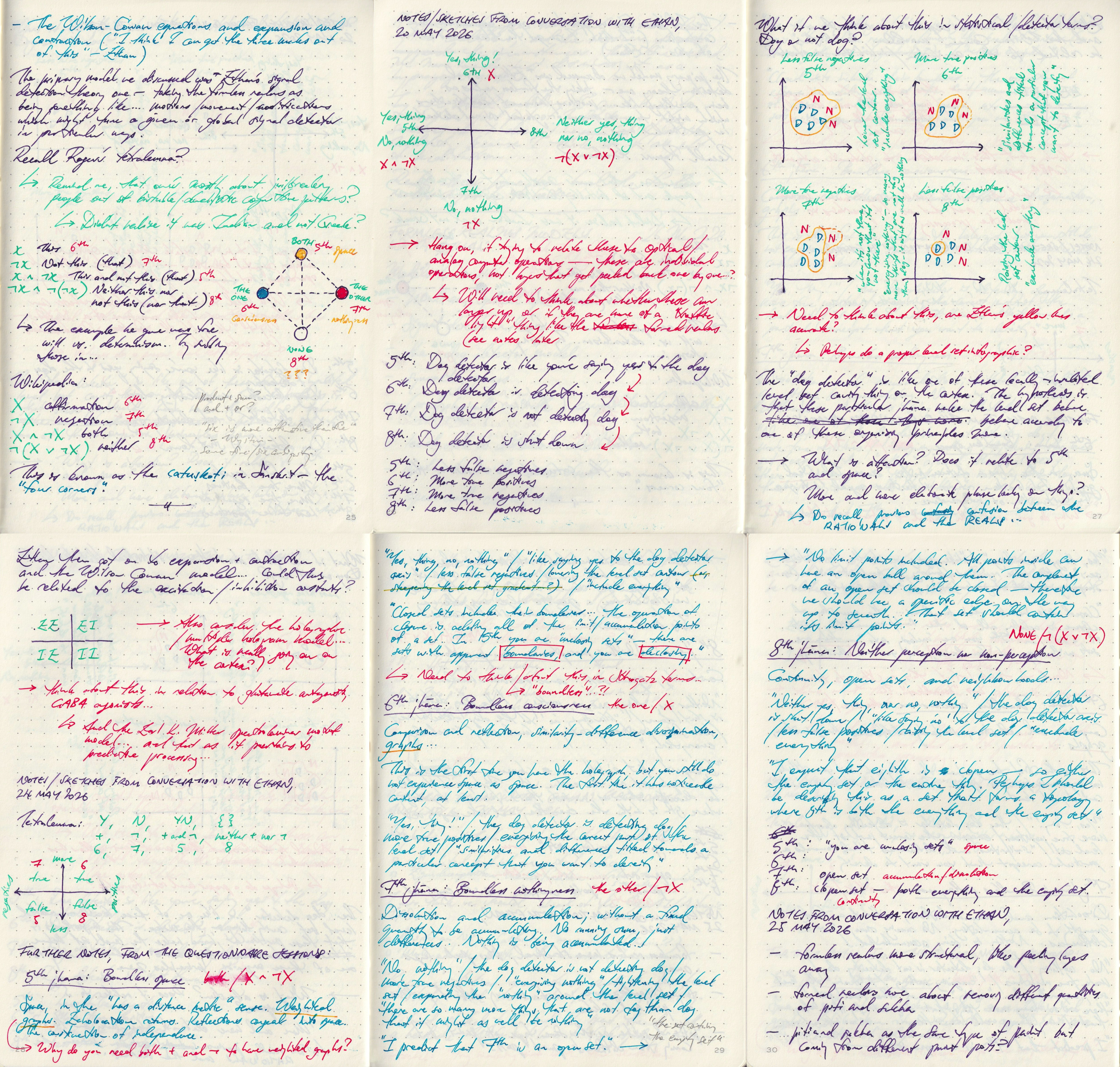
Sketches exploring models of the formless jhāna, summarising many hours of infodumping.
In this section, I shall run through six models of the formless jhāna that we discussed. Once again, let’s put these models side by side to see if any patterns appear.
We’ve already discussed the idea that traversing J8 to J5 may be equivalent to adding instructions one by one to the instruction set of a hypothetical analog computer, but I’ll review our proposal again briefly, in ascending order this time:
Starting with J8, the first computational property we add is connectedness, which is a reasonable prerequisite for basically anything else. Then with J7, people report a sense of nothingness – but when prompted, they cannot report on how much actual nothingness they are experiencing, only whether the amount of nothingness is increasing or decreasing – there’s no running sum. Might this correspond to supporting the ability to observe change over time in the form of a first derivative – while yet still lacking the ability to compare absolute values? With J6, we do add the ability to compare constructs and their absolute values, and with that a sense of self-reflective consciousness or metacognition finally forms, along with the notions of similarity and difference. Everything starts to reflect everything else. Then with J5, we use this capability to compare locations of points in space, establishing a distance metric, and with that a sense of – typically three-dimensional – space finally congeals, which is experienced as a contentless volumetric holograph. The graph of experience becomes a weighted graph at last.
What kind of “analog instruction set” should we expect the general class of analog computers to typically implement? The MONIAC – a hydraulic computer devised in 1949 to teach students at the London School of Economics about the economy of the United Kingdom – is very good at integration, for example.
How could we tell that this model is correct? Ethan has a number of ideas. Perhaps if you hang out in J5 for a really long time you’ll notice that your brain becomes really good at rendering a sense of space cheaply with minimal accompanying tension – and if you spend a lot of time in J6 you could become very good at performing fine-grained mental comparisons of quantities like relative distances or amplitudes. You might get better at hue distinction – there’s even online games which can test this sort of thing. J7 and J8 might be outright cognitively impairing – Ethan speculated that in J6 the stuff-to-things axis inclines towards things, but in J7 it inclines towards stuff – and in J8 this axis comes apart entirely. This squared with what Wystan reported:
Wystan: If I’m spending a bunch of time in the formless realms and then I get up, my proprioception is kind of fucked. I might bump into something. Seems to resolve itself pretty quickly.
He also explained to us how monasteries which accommodate deep insight practices also have to accommodate changes to people’s cognitive abilities:
Cube Flipper: You mentioned to me other day how some monks might spend an excessive amount of time in highly defabricated states – and thus be excused from doing the dishes?
Wystan: Yeah, they literally develop functional deficits if they do that sometimes. Especially people who do extended dark retreats – that’s infamous for this. Some people will spend years in dark retreat, and they come out with social, motor, cognitive deficits – and sometimes they don’t get all their functioning back.
Cube Flipper: So – don’t ask a perfectly spherical monk to do your dishes.
Wystan: No, I mean, a Zen monk will do your dishes damn good. Probably better than anyone else.
Cube Flipper: Oh, because the Zen monks actually practice folding back up again!
Wystan: Exactly.
I guess we might not know for sure how all this works until we do get the chance to run some psychophysics tests on formless jhāna meditators – perhaps there is a tradeoff happening between general and specific cognitive faculties, which is reasonably overlooked by people in a monastic setting. Otherwise, I think this broadly makes sense – if you shut down most of your computer’s processes, obviously you should expect to get worse at computing.
Wystan: Anecdotal personal experience, but coming out of J4 is pretty optimal for pretty much any task. This is why it’s so good for insight practice – but why it’s good for insight practice is why it’s good for any task.
We started this project focused on the computational properties of the jhāna, but as I completed my interviews with the retreat participants, it became clear to us that perhaps group theory could provide a more foundational model. As I wrote, in The third QRI psychophysics retreat, part II: The formless jhāna:
I think that if we walk backwards from cessation all the way to waking consciousness, then we can characterise the transitions through the jhāna as a series of symmetry breaking events as more and more degrees of freedom are added. It follows from this that we should then be able to characterise the formless jhāna by their corresponding symmetry groups – as Mike Johnson has proposed before. To provide a concrete example – if someone reports that the only thing remaining at J8 is the sense of time, we can use this type of claim to narrow down the set of groups which might describe J8.
If we can observe those same symmetry groups in neuroimaging data – perhaps with a specific focus on the difference between cessation and J8 – this might then take us one step closer to finding the correlates of consciousness, and ultimately how the structure of waking consciousness itself comes to arise.
The full story is written up in that post – it’s quite complex, and group theory is kind of opaque, so if the reader finds it confusing I think it’s reasonable for them to skip this section. Anyhow, given the small cohort size and sparsity of reports – only three participants could reliably reach the formless jhāna – I remain hesitant to propose concrete mappings between jhāna and specific symmetry groups. Here’s what I was prepared to say:
J5: Space: E(3), Sim(3) or Aff(3); time: ℝ, E(1), Aff+(1), or Aff(1)
Ethan also proposed that the bare-bones structure of the formless jhāna could be understood in terms of set theory. I’ll outline the mapping before we attempt to justify it phenomenologically:
J5: The set containing both the empty set and the set containing the empty set, {{∅}} ∪ {∅} = {∅, {∅}}
J6: The set containing the set containing the empty set, {{∅}}
Ethan:J8 is self-explanatory. In J7, there’s nothing but a hint of nothing. You’re the set containing the empty set – you can sense the empty set – under a very refined concept of sensing. You’ve got something like a gigantic bubble, and inside this bubble is practically vacuum, and the bubble has negligible tension, and that’s it.
I found it interesting to note that given his mathematical background, Ethan actually thinks of these things spatially – when he imagines the set containing the empty set, he actually does imagine something structurally similar to J7. By comparison, I’m just a hapless wordcel, envisioning symbols on the whiteboard of my mind’s eye. Ethan tells me that thinking this way may be more intuitive if you deeply internalise the axioms of topology.
Since each set is constructed from other sets, you can relate each set to its children using a directed graph structure. Maybe there’s a hint in here as to how I should structure my formless jhāna symmetry group lattices.
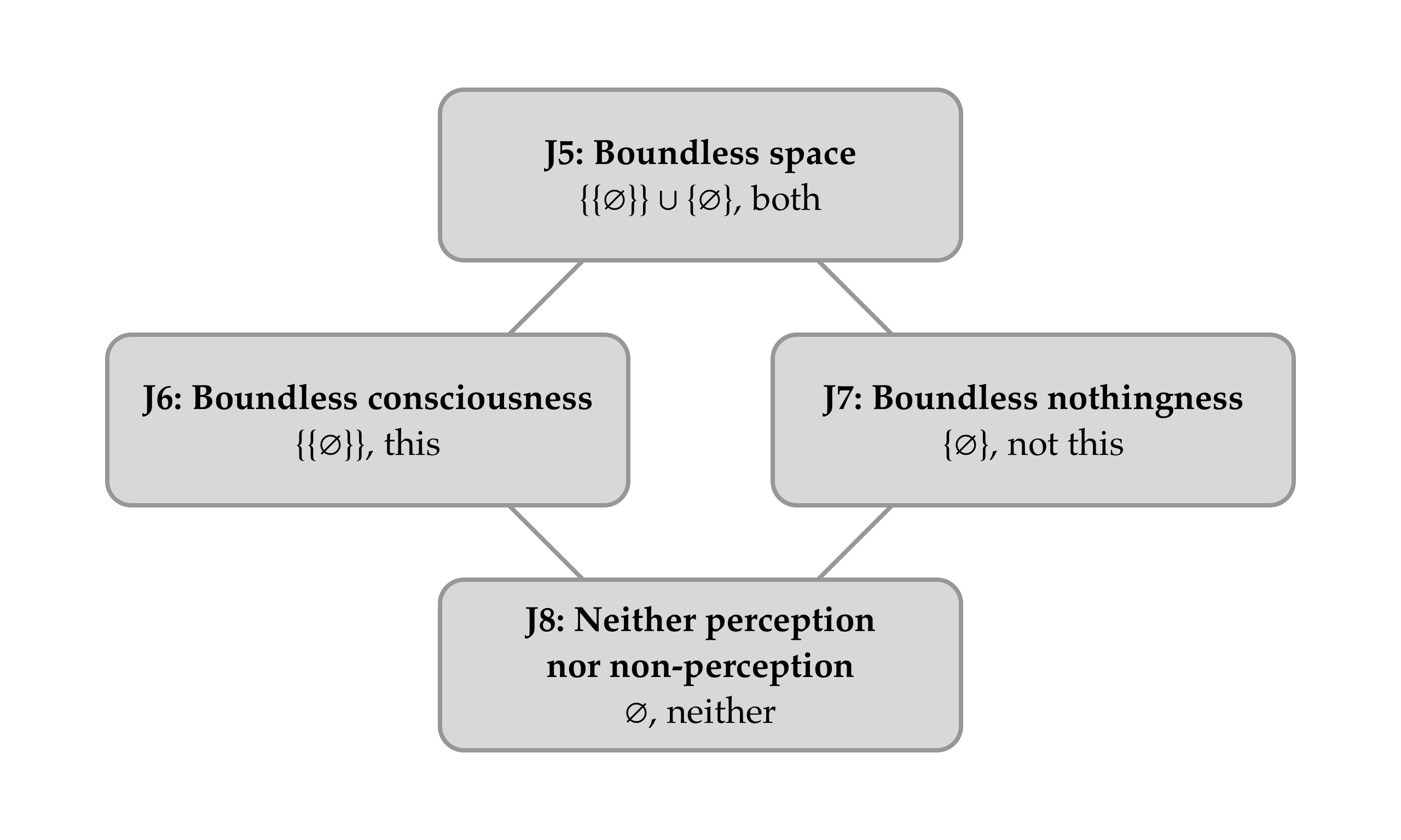
J5: The set containing J8 and J7 – or equivalently, the union of J6 and J7
If this is the case, then these four jhāna form a diamond:
Formless jhānaHasse diagram. J5 forms the union of J6 and J7, which are incomparable – neither is a subset of the other – and J8 forms their intersection. Or, join and meet, if you prefer that terminology. This also nicely matches the shape of the tetralemma, as we shall see later.
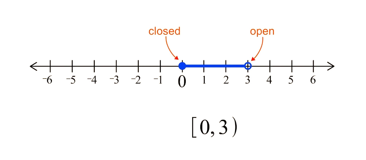
Sets can also be understood in terms of points and neighbourhoods. We say a set is closed when it includes all of its own edges – if every neighbourhood of a point contains some points of the set, then that point belongs to the set. We say a set is open when it includes none of its own edges – so every point in it has a neighbourhood entirely inside the set.
Imagine a number line – the standard convention is to show a hollow circle at an open endpoint which is not included in the set; and a solid circle indicates a closed endpoint which is included in the set:
The way these sets handle points and neighbourhoods describes the relationships between the atomic components of experience in the corresponding jhāna. Perhaps J5 and J6 will make more sense this way:
J5: Clopen. All points have neighbours. Space has formed, and like the entire number line ℝ, there is no edge anywhere.
J6: Closed, nowhere dense. All edge. Space is yet to form. Points exist, but their only neighbourhood is the entire space. No point has a local neighbourhood of its own.
J7: Open. All neighbourhood. Like an open interval, it approaches its edges without ever reaching them, so there is no endpoint to measure from – only a direction of travel.
J8: Clopen. There are no points. Only topology is preserved, the rules for what points would neighbour what.
In the abstract version of this model, J5 is everything – the whole space. It splits into the complementary sets J6 and J7 – a set made entirely of boundary, and a set which stops just short of its boundary. Take their union and you get J5 again – and take their intersection and you get J8 – nothing.
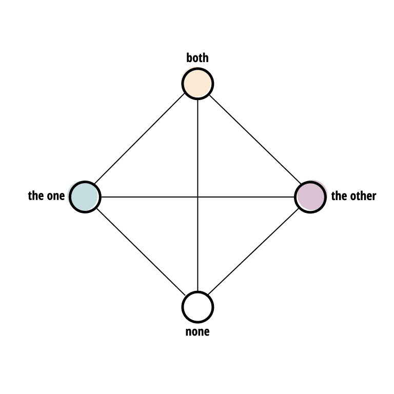
You may have spotted that the set theory pattern reduces nicely if you read the four sets as the four subsets of {yes, no} – both, this, not this, neither. This should look familiar to anyone acquainted with Indian logic – this is the catuṣkoṭi, or tetralemma, which admits four possibilities for a proposition P:
I felt there was a potential correspondence between the four corners of the tetralemma and the void, unit, sum, and product of algebraic data types – but there were several viable ways of making it work, so I decided to leave it for now. It’s a shame – a working type theory sure would impart some useful computational properties.
Earlier, we observed the form jhāna to follow the sequence, pīti, both pīti and sukha, sukha, neither pīti nor sukha – which maps straightforwardly onto the tetralemma. However, if we follow the classical order of the tetralemma, both the form jhāna and the formless jhāna visit all four corners, but in different orders, J1-J3-J2-J4 vs. J6-J7-J5-J8:
Affirmation: J1pīti, J6this
Negation: J3sukha, J7not this
Both: J2both pīti and sukha, J5both this and not this
Neither: J4neither pīti nor sukha, J8neither this nor not this
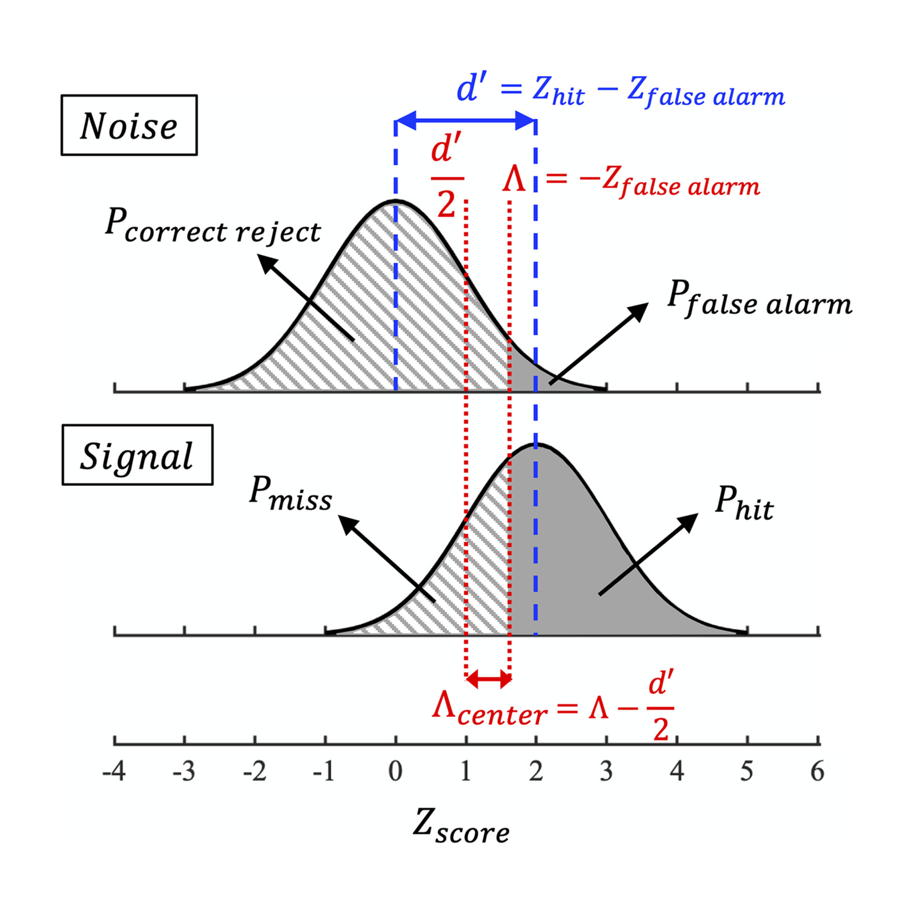
The tetralemma is abstract – how do we make it concrete? Signal detection theory presents a natural answer. Let’s say you are trying to tune or train a signal detector to tell signal from noise. For any given input, there’s four possible outcomes – hit, miss, false alarm, and correct rejection:
A diagram showing the four possible outcomes from signal detection theory. The way I mentally visualise it, when tuning your signal detector you are trying to maximise the area of Phit and Pcorrect reject while minimising the area of Pmiss and Pfalse alarm. Illustration from Circadian and Visual Neuroscience.
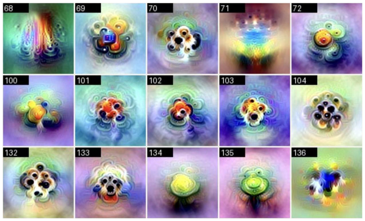
These of course map nicely onto the tetralemma. What if the jhāna correspond to sinking your attention into these four possible outcomes? To make things more visual – since real world situations are much higher dimensional than these one dimensional Gaussians – Ethan and myself liked to talk about this in terms of a hypothetical dog detector. Imagine some collection of neurons, perhaps somewhere in the ventral stream, which activate when a dog is present in the visual field – either correctly detecting dog or not dog, or registering a false positive or false negative.
Feature visualisations of dog detecting neurons in a convolutional neural network, from OpenAI Microscope via Nick Cammarata.
Ethan proposed that the formless jhāna are a bit like encouraging such a dog detector to adjust its behaviour – but the global equivalent thereof:
Ethan: So, some concepts are very natural, right? Like, dog – very natural concept. So this is a very important axis that basically all of your categorizations are going to have. How natural is this abstraction that your’re making?
Ethan: Pretty much the key thing would be that for any concept that you’re entertaining, you can take it for granted that you’re going to ask – how much is this thing pinging this concept detector? How dog is this thing that I’m looking at? Then you also have – do I think this thing is a natural concept? I’ve got all this stuff that’s getting wrangled together into something saying, these things co-vary, and share natural features and so on – but how natural is this concept, really? This can vary a great deal, where you have super terrifically natural concepts – take ball, that’s a crisp one – and then we have some arbitrary baroque thing which is never going to come up again.
Wystan:Post-colonial glaciology.
Ethan: We can do worse! So quite often I’m thinking about both of these at the same time – how natural is this abstraction for this thing that I’m looking at, and also is this thing in this category or not. So for the dog detector – if the dog detector is becoming less of a dog detector, then you don’t believe in dogs so much as an abstraction anymore.
This results in the following mapping:
J5: The dog detector is more of a dog detector, more false positives, false alarm
J6: The dog detector detects dog, more true positives, hit
J7: The dog detector does not detect dog, more true negatives, correct rejection
J8: The dog detector is less of a dog detector, more false negatives, miss
Now generalise from one detector to all of them at once – could this be what generates the formless jhāna?
There exists a nice way of visualising signal detectors, using something called level sets:
Cube Flipper: Can we explain level sets quickly?
Ethan: Say you’ve got a topographical map. The level set for fifty feet off the ground is just the slice corresponding to that contour.
Cube Flipper: Right. So imagine there’s a state space of a signal, and your statistic is a level set over some chunk of that space – and tuning the dog detector reshapes the level set.
Every detector – even if it is operating in a very high dimensional space – is just a function that draws a line across its input space. Let’s say we keep that threshold fixed in place – what if the jhāna correspond to four linear operations you can apply to the input space?
So J6 and J7increase and decrease discriminatory potential, respectively, while J5 and J8lower and raise the threshold waterline.
I like this model because it works equally well in both signal space and cortical space. One hypothesis we have yet to spend time exploring is that instead of abstract level set topography we might be talking about actual oscillatory processes on the cortex – and instead of an arbitrary threshold, you’d get to use the natural nodal lines separating regions in phase and counterphase.
For now, Ethan tells me that in order to wrap my head around the computational properties of this class of system, I will need to know more about Reeb graphs and Morse theory – but I’ll be the first to confess that my brain is now at capacity so far as models of the jhāna go, and I shall have to let things percolate in the background for a little while before I return to this problem.
I hope you enjoyed the post. We enjoyed putting it together for you.
Throughout the 2010s, I very much enjoyed reading the consultancy blog Ribbonfarm, written by Venkatesh Rao and a cast of guest writers. I found their unattached, flippant attitude towards model building to be a refreshing alternative to the neighbouring rationalist community which was my otherwise default home turf.
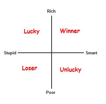
One Ribbonfarm ingroup joke was the concept of the 2x2, or quadrant diagram – a PowerPoint slide staple, it’s a natural way to present a two-axis carving of an arbitrary concept space. There’s an art to these – as he says, in How to Draw and Judge Quadrant Diagrams (2009):
The quadrant diagram has achieved the status of an intellectual farce. If you, as a presenter, do not make an ironic joke when you throw one on the screen, you will automatically lose a lot of credibility. For some very good reasons though, the diagram is an indispensable one for the presenter’s toolkit. As a listener, if you have a default dismissive attitude towards the thing, you will have to sit out far too many important conversations with a cynical, superior smile. So here’s a quick tutorial on quadrant diagrams. I’ll tell you both how to make them, and how to evaluate them. Here’s a made-up one to get the basics clear. You basically take two spectra (or watersheds) relevant to a complex issue, simplify each down to a black/white dichotomy, and label the four quadrants you produce, like so:
This particular one is nonsense, and falls apart at the slightest poking (we’ll poke later in the article), and I made it up for fun.
I did not use any quadrant diagrams in this post, though I easily could have – the jhāna are a natural candidate, given – well – there’s four of each kind. Maybe the attentive reader found themselves sketching their own quadrant diagrams on their mental whiteboard while reading the text, in order to efficiently compactify the ideas presented. We’re still not fully committed to any of the ideas in this post, so I think we should reserve any quadrantology for now. Consider these ideas held in suspension, ready to crystallise when the time comes for us to pick up this project once again. In the meantime, if you are someone who can both jhāna and discuss abstract mathematical models of experience, we’d love to hear from you.